


The Ambisonic Technique
What’s in a Name?
In large part, the techniques and technologies grouped under the name “Ambisonic” can be traced back to the late 1960s and early 1970s experimentation with sound recording of Michael Gerzon and his colleagues in the Oxford University Tape Recording Society (OUTRS). I think it’s useful to begin by remembering this, as most contemporary music audiences (and composers) consider Ambisonics to be just another “surround sound” technology in a panoply of competing approaches (Wavefield Synthesis [WFS], Ambiophonics, Binaural, 5.1, 7.1, etc.). Similarly, most audiences identify Ambisonics with colorful synthetic sound textures. When the word appears in a concert program note, we often expect to hear electronically generated sounds flying through the performance venue. And certainly this was the case at the Warsaw Autumn 2009 International Festival of Contemporary Music for the audience hearing music from Seattle’s DXARTS presented at the Extra-High Voltage Hall. In origin though, the interest of the creators of Ambisonics was clearly to come up with a way to accurately capture, record and then reproduce a naturally occurring musical performance or soundscape.
As a composer of electroacoustic music, I’m quite interested both in making and hearing abstract sounds take to the air and flutter about space. 1 That said, beginning with this notion of natural sound recording can help us to understand the design philosophy and advantages found in the Ambisonic approach. From this view, Ambisonics seeks to capture a naturally occurring soundfield in three dimensions. 2 The picture found in Figure 1 illustrates an arrangement of microphones deployed by OUTRS intended to do this – we need four microphones to capture sound in three dimension. Using technical language, we’ll call this capturing “soundfield sampling.”
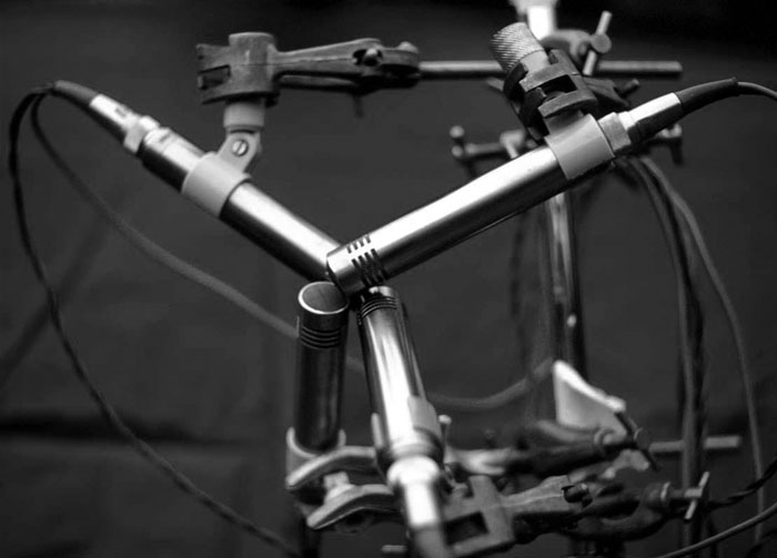
Figure 1: OUTRS tetrahedral microphone array, courtesy Stephen Thornton (www.michaelgerzonphotos.org.uk)
The OUTRS microphone array may appear to be intuitive, but I shouldn’t fail to mention Gerzon was a mathematician at Oxford’s Mathematical Institute, as were a number of his OUTRS colleagues. So, Ambisonics developed through both practical experimentation and theoretical grounding. We’ll look at playback and modifications to the soundfield later, but our starting point is the notion that we can somehow record and capture the spatial features of a real acoustic event.
Turning to the word “Ambisonic,” the prefix “ambi” means “around.” From this root comes the word ambient for which two definitions are useful: existing or present on all sides; an encompassing atmosphere. Of course “sonic” is of, or involving sound. Simply put, “Ambisonic” is a word coined in the early 1970s to describe this powerful approach to “surround sound.” I’d like to pay particular attention on the second notion of ambient, an encompassing atmosphere, for this is a very important concept for the Ambisonic technique which hopefully will become more clear in this brief discussion.
Soundfield sampling: capturing sound
While it is completely possible for a contemporary sound engineer or electroacoustic composer to make recordings using a tetrahedral microphone array as per the experiments in Oxford four decades ago, I can’t say this is especially convenient. To be accurate, the four microphones really should be quite carefully aligned. The solution to this problem came with the development of the Soundfield microphone by Gerzon and Peter Craven in 1975. If we look inside a contemporary microphone manufactured by SoundField Ltd., Figure 2, we’ll see four microphone capsules arranged tightly in a tetrahedron. As you can imagine, this is a much more precise alignment than is possible with separate microphones. Additionally, aside from the strict geometry, the soundfield microphone includes further electronics to additionally tighten the resulting sampling of the soundfield to be captured.

Figure 2: Soundfield microphone capsules, courtesy SoundField Ltd. (www.soundfield.com)
If we ask the question “Why four microphones?,” the answer comes fairly quickly. Think back to your school geometry lessons: two points allow us to define a line, which has a single dimension; three points define a plane, two dimensions; and we need four points to define a volume, three dimensions in space. Though easy to understand, this is in some way a simple and naïve explanation. Soundfield sampling is the technical description: acousticians characterize the action of the soundfield microphone as “spherical harmonic soundfield decomposition.” The mathematics of this sampling operation has associated degrees of accuracy. For a minimum three-dimensional representation we need at least four microphones, which gives us four “spherical harmonics.” Later, we’ll see that we can use more than four, but our minimum is four.
Back to being more intuitive, it is dividing space up into pieces, like we divide up a cake or pie to serve. Each microphone captures different “slices,” therefore together they gather up a complete picture of the sounds occurring around the soundfield microphone. We grab an all-encompassing picture of the world of sound around us, the natural “soundscape.” I think of it as is illustrated in Figure 3, with this process resulting in a representation of the captured soundfield in a form called “B-format.” With an encapsulated natural soundscape on hand, the composer then has the opportunities of a sculptor to reshape, remould and reform the spatial characteristics of sound. This is where Ambisonics is strikingly different from the other surround sound technologies mentioned earlier.
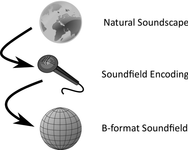
Figure 3: Soundfield recording
B-format techniques: reshaping space
It is difficult to overemphasize the creative power Ambisonic soundfield processing techniques bring to the composer. This is in large part due to the fact the whole soundfield is represented, rather than individual elements placed in a space. Whole space, the entire ambience is encapsulated in B-format. Once the composer has complete “picture” of a sound world or soundscape, that picture can be rearranged, distorted, warped or re-imagined otherwise.
Soundfield Rotation
Most discussions of B-format processing techniques start with a set of “imaging transforms” known as “rotations.” As you might imagine, rotations allow one to re-align a B-format soundfield. There are different names for these depending on which axis in Cartesian space the soundfield is rotated across. “Tilt” is illustrated in Figure 4. Rotations preserve the complete soundfield, and are equivalent to re-aiming or “steering” the microphone in the original recording space. For the sound engineer, rotations are very useful for remedial purposes: once back in the studio a misaimed microphone can be corrected, perhaps to center an off-kilter string quartet.

Figure 4: Soundfield tilt
Depending on the context, I tend to think of rotations in two different ways. If the B-format recording is of a very full and vibrant natural soundscape, I tend to see the imagine rotations as if I’m turning my head, listening to a re-orienting soundscape. Imagine a day at the seaside with ocean waves in the distance, children playing in the mid-field, seagulls above, and a barking dog in the near-field. Think of the children playing, turning their heads as they play dancing on the beach: as they turn, the soundscape rotates around them.
With isolated sounds recorded in a sound studio, I tend to view rotations as applying motions to sounds, moving them through space. So, rather than giving the sense of the listener changing his or her orientation within a soundscape, individual sounds recorded and then transformed in this way appear to change their relationship with the listener. To get this suggested sense of motion, the composer needs to be changing the applied rotation in time. Interesting things happen while rotating at different rates across several axes at once–In my toolbox of techniques I call this “twirl.”
Soundfield Warping
The next two groups of B-format processing techniques result in some sort of warping of the spatial dimensions of a captured sound. What I call “push,” “press,” and “squish” principally act by distorting the arrangement of the sounds captured in a B-format recording (those falling in the category of “dominance” techniques [described below] also change the balance between individual elements). In my view, the warping techniques are where much of the leverage for the composer working with Ambisonics is to be found. These are the tools that allow the composer to act as a spatial sculptor – not only to compose in space, but to compose and re-compose space.
The illustration of squish found in Figure 5 offers an example of the kinds of results possible and gives the sense of the recorded soundscape being somehow flattened through an axis. As with sculpture with physical materials, like e.g. stone, wood or metal, the resulting impression varies considerably depending on the starting sound’s material. Warping an active soundscape, like our beach example, gives a completely different impression than warping a single sound recorded in the studio.
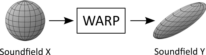
Figure 5: Soundfield warp (squish)
Push and press will warp and compress a soundfield in a particular direction. Push maintains the soundfield as a sphere, where press warps as a flattened spheroid. By warping our beach soundscape with press changing in time, it is possible to create a kind of “spatial bloom:” blooming or expanding out the soundscape from a single point to expand and fill out space, as did our initial B-format recording. I use this technique extensively in my own work to create blooming sounds and soundscapes, particularly in “Mpingo” and “Pacific Slope.”
Dominance
Along with rotations, “dominance” is one of the first transforms to have been introduced as an Ambisonic processing technique, and has been included as a control on the high-end soundfield microphone models.3Sometimes the name “zoom” is used, as one impression of this effect might be described as zooming into a soundscape – just like a zoom lens on a camera zooms into a landscape. Dominance can be implemented in slightly different ways, giving somewhat different results; but at the heart of it, what is happening is that the balance in volume (loudness) between different parts of the B-format soundfield is adjusted. A simple way to think of this is that we are adjusting the volume between the four microphones that initially sampled the soundfield. Of course, it is more complicated than this, but that’s the idea.
Another way I think of it is going back to our slices of pie. At one extreme, dominance allows us to select, or “focus,” on one slice of pie. The dominance effect is continuous, so we can slowly vary the balance between the various slices. Imagine focusing on sound in a single direction, say front, then slowly expanding, adding in the missing slices of pie so that the perspective expands. With our beach soundscape example, we could start with the slice containing the playing children. Then, slowly build up and complete the whole space, finally engulfing the listener with the surrounding seaside soundscape. As you can imagine, along with the previous effects, this gives a great deal of creative control to the composer.
Spatial Aliasing
Within the technical literature, aliasing usually refers to “misidentification of a signal” or “introducing a distortion or error.” While we might imagine such a thing could be useful from a musical perspective, “a false or assumed identity” is the definition I find most valuable in my thinking as a composer. For the sound recordist and acoustician, “spatial aliasing” is usually something to be avoided, the ideal being an accurately captured soundfield (the four-capsule soundfield microphone was actually designed to dispense with the spatial aliasing problems found in OUTRS tetrahedral microphone array.)
For the composer though, “a false or assumed identity” – ambiguity – can be a powerful part of a composition language. Within the history of Western Art Music we’ve seen that tonal ambiguities have become an important device in the expressive palette available to musicians. With spatial aliasing techniques we can bring similar approaches to space: at one pole sharp, vivid and well-defined pictures; on the other – vague, indistinct, hazy or drifting. Envisage a clearly defined scene slowly evaporating and losing form – or the other direction, a vivid world condensing from a foggy expanse. Because B-format gives a representation of the soundfield, the composer can apply a number of different techniques to create various types of aliasing resulting in a variety of different impressions.
Soundfield Mixing
At first glance, it might seem rather strange to propose “mixing” as a powerful soundfield technique. A number of the surround sound approaches listed at the beginning of this discussion, in particular Wavefield Synthesis, are best regarded as “auralization” technologies. For our purposes, auralization is a way of modelling space, and then simulating a placement of sounds in that space in relation to a modelled position of a listener. We can use Ambisonic technology to do this modelling and, interestingly, quite a number of auralization systems do that (including computer gaming systems as well as for concert hall design). However, the use of Ambisonics for simple auralization doesn’t really take any advantage of the powerful techniques described above.
Additionally, we can mix together and overlay a number of complete and complex soundfields, creating new, very dense and complex soundscapes. This is exactly the approach the composer Ewa Trebacz has taken to make her Errai, premiered at the DXARTS concert mentioned earlier. Trebacz placed a soundfield microphone in a large, reverberant cistern and recorded performances of soprano Anna Niedzwiedz and horn player Josiah Booth. Then she did this again, and again, and again. Finally, she mixed together the resulting soundfields as illustrated in Figure 6. The result is an acoustically realistic, but dense and fantastic all-encompassing soundscape: ultra-magnified ambience. Here, the layering of space itself becomes a compositional technique.
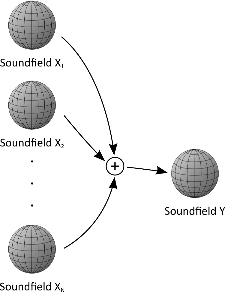
Figure 6: Soundfield mixing
Soundfield reproduction: playing back
The astute reader familiar with surround sound systems will recognise that I haven’t actually discussed the number of loudspeakers Ambisonics uses for playback. Ambisonics is very interesting in that it doesn’t involve channels the way we’re used to thinking about them. Soundfield recording (or synthesis) and playback are two separate activities, that is, they’re completely decoupled. Figure 7 illustrates the situation. Once we have a soundfield in B-format, we need to “decode” it to translate the spherical harmonic representation of the soundfield for audition over loudspeakers (or headphones.)

Figure 7: Soundfield playback
This idea of decoupling the soundfield representation is a part of the enlightened design of Gerzon and his contemporaries. B-format represents a fully three‑dimensional soundfield – how we finally listen to it is our choice. The process of decoding translates our soundfield to the number of loudspeakers we’ve selected to play back on. We can decode to two-channel stereo 4 or for binaural headphone listening5. We can decode to four loudspeakers for compatibility with “quadraphonic” surround sound systems. Similarly, we can decode for modern 5.1, 7.1 or other arrangements.
As B-format is fully three-dimensional, composers can playback over full 3D systems, with loudspeakers placed above and below the audience, giving a fully immersive, completely 3D experience. The audience at the Extra-High Voltage Hall was treated to playback over twelve loudspeakers, a ring of six above and six on the floor. My Ambisonic studio at the University of Hull, shown in Figure 8, uses two rings of eight plus another four subwoofers; a 16.4 fully 3D surround system. Other arrangements are certainly possible, so that another advantage of Ambisonics is the number of loudspeakers for playback can be chosen as performance conditions require – a real boon to composers.
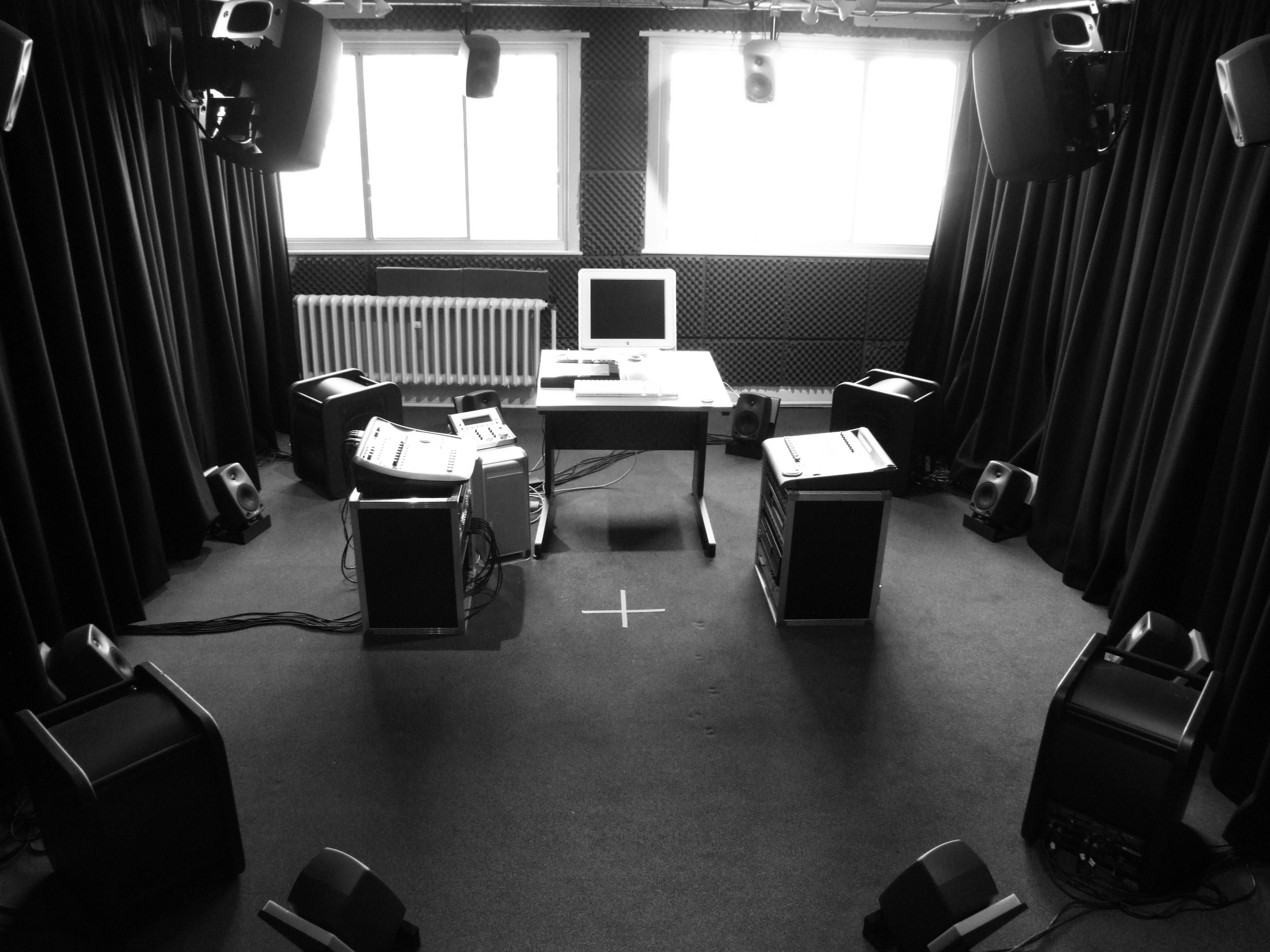
Figure 8: Ambisonic Studio, University of Hull
The cutting edge: Higher Order Ambisonics
We’ve seen that Ambisonics, having been with us as a technology since the early 1970s, is quite mature. So, what’s new, then? Strangely enough, in a number of ways we can regard recent developments in the area of Wavefield Synthesis to have spurned on further research in what is called Higher Order Ambisonics (HOA). If you recall the pie slicing metaphor we used to describe soundfield sampling, you’ll remember we used four microphones to translate into B-format, our spherical harmonic soundfield decomposition. As you might expect, we can use more than four to get finer slices, and therefore a more accurate representation. Increasing these slices – our accuracy – is described as increasing the “order” of the spherical harmonic sampling (see Table 1: Ambisonic Orders).
Table 1. Ambisonic Orders
| Ambisonic Order |
Number of Spherical Harmonics |
| 1 | 4 |
| 2 | 9 |
| 3 | 16 |
As a composer I’ve been quite happy to work with first-order B-format, but the increasingly accurate soundfield available with HOA gives progressively more focused and stable images for a wider audience, leading to greater expressive possibilities. That is, HOA gives higher spatial fidelity and sharper realism. Additionally, it is interesting to know that the mathematics for HOA and Wavefield Synthesis have been shown to be equivalent – solving the same problem given different starting points.
It turns out that more is involved with HOA than just adding extra microphones, and HOA microphones are a developing area of research. A number of designs have been proposed, a few experimental arrays constructed, but at the time of writing I’m aware of only one periphonic (fully 3D) HOA capable microphone on the market, mh acoustic’s “Eigenmike” (Figure 9). I’ve listened to both synthetically produced HOA soundfields6 and experimental recordings made with the Eigenmike. As you’d expect, both experiences leaving a strong impression. To my knowledge though, no composer has as of yet had access to HOA recordings made with the Eigenmike. In my mind, this is to be the future of musical work with Ambisonics – HOA using all the techniques and opportunities for expression described above.
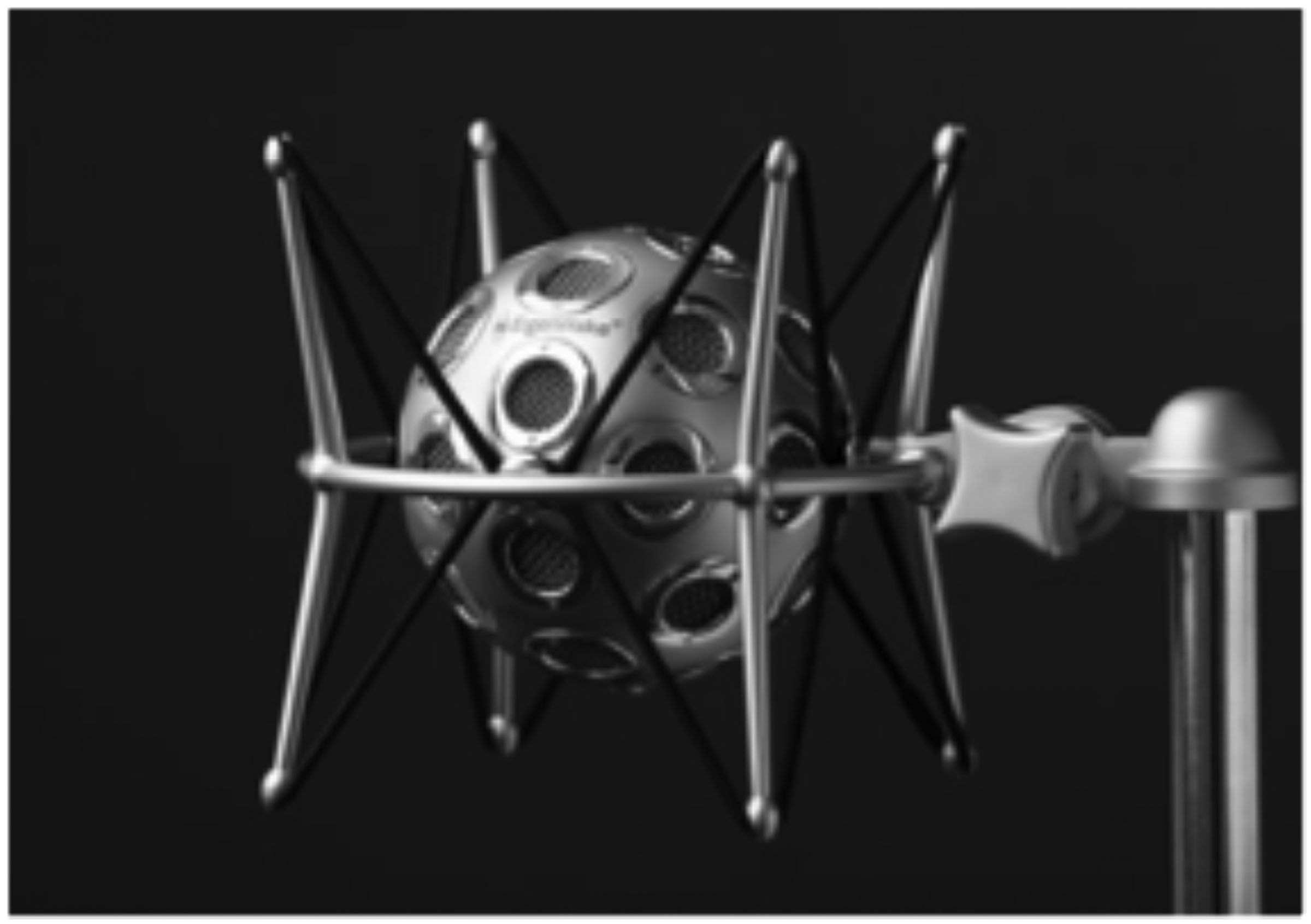
Figure 9: Eigenmike, mh acoustics LLC (www.mhacoustics.com)
I first came to the United Kingdom to study both composition and the art of “sound diffusion” with Jonty Harrison. Denis Smalley has described sound diffusion as “the projection and the spreading of sound in an acoustic space for a group of listeners, as opposed to listening in a personal space (living room, office, or studio).” Another definition would be the ‘sonorizing’ of the acoustic space and the enhancing of sound-shapes and structure in order to create a rewarding listening experience. ↩
In the technical literature, the word ‘periphonic’ is used: ‘Peri’ for surrounding and ‘phonic’, sound. ↩
The SoundField, Ltd. model MKV includes dominance. ↩
Nimbus Records’ stereo recordings are Ambisonic. ↩
Auralization systems often use this binaural route. ↩
A few composers, Natasha Barrett and Jan Jacob Hofmann included, have experimented with composing music using HOA. ↩